Here we will describe a probabilistic approach to solving
equation (1.6). For simplicity let us
consider the case when the forcing term
![]() .
We will not be rigorous.
.
We will not be rigorous.
We will
suppose that we have found ![]() using equation (1.5).
Now let
using equation (1.5).
Now let
![]() be a Brownian motion in 3 dimensions, starting at
the origin. Define
be a Brownian motion in 3 dimensions, starting at
the origin. Define
![]() .
Let
.
Let
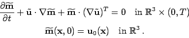
![]() be a random vector field that satisfies
the equations
be a random vector field that satisfies
the equations
The reason why this works is because of the Itô formula. We have
that
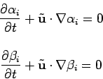
The solution to equation (6.1) can be computed as
follows. Suppose that the initial value of ![]() satisfies
equation (1.3). Then if
satisfies
equation (1.3). Then if
This can be used to obtain the following plausibility argument for the
regularity of the Navier-Stokes equations. Let ![]() denote the
space of functions from
denote the
space of functions from
![]() for which minus one derivative is in
the space of functions of bounded mean oscillation. It is known that the
space
for which minus one derivative is in
the space of functions of bounded mean oscillation. It is known that the
space
![]() is a critical space for proving
regularity for the Navier-Stokes
equations (see below). That is, if one can show that the solution to the Navier-Stokes
equations is uniformly in time in any space better than
is a critical space for proving
regularity for the Navier-Stokes
equations (see below). That is, if one can show that the solution to the Navier-Stokes
equations is uniformly in time in any space better than ![]() (such as
(such as
![]() for any
for any ![]() ), then the solution is regular.
), then the solution is regular.
Now if the initial data are very nice, then by using some partition of unity
argument, we may suppose that indeed the initial value of ![]() does satisfy
equation (1.3) for some finite value of
does satisfy
equation (1.3) for some finite value of ![]() ,
where the initial values of
,
where the initial values of ![]() and
and ![]() are compactly
supported smooth functions. Then it is easy to see that the solutions
for
are compactly
supported smooth functions. Then it is easy to see that the solutions
for ![]() and
and ![]() provided by the transport equations stay
uniformly in
provided by the transport equations stay
uniformly in ![]() . Thus it follows that
. Thus it follows that
![]() is uniformly
in the space
is uniformly
in the space ![]() .
.
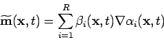
Thus
![]() is a finite sum of a product of functions uniformly in
is a finite sum of a product of functions uniformly in ![]() and functions uniformly in
and functions uniformly in ![]() . Thus it might seem that we
are close to showing that
. Thus it might seem that we
are close to showing that ![]() (which is the Leray projection of an average
of translations of
(which is the Leray projection of an average
of translations of
![]() ) is in a space that is critical for proving
regularity.
) is in a space that is critical for proving
regularity.
There are some large, probably insurmountable problems with this approach.
The lesser problem is that we need a space that is better than critical.
The bigger problem is that the space created by taking the convex closure
of products of bounded
functions and functions in ![]() is not really a well defined
space, in that it encompasses every function.
is not really a well defined
space, in that it encompasses every function.
Criticality of
![]() : Let us present a
formal proof of this fact, in the case of the Cauchy problem with zero
right-hand side.
Let
: Let us present a
formal proof of this fact, in the case of the Cauchy problem with zero
right-hand side.
Let ![]() be the solution to the Navier-Stokes
equations which belongs to the space
be the solution to the Navier-Stokes
equations which belongs to the space
![]() . Multiply equation (1.5)
. Multiply equation (1.5)![]() by
by
![]() and integrate over
and integrate over
![]() . Notice also that
. Notice also that