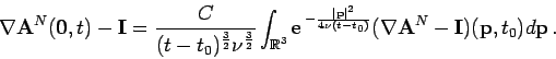
Let us now look in particular at
![]() for
for ![]() . We have that
. We have that
![]() satisfies the heat equation
satisfies the heat equation
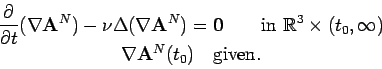
Therefore also
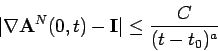
Our first goal will be to show that the function ![]() in Lemma 2.2
satisfies
in Lemma 2.2
satisfies
![]() as
as ![]() uniformly in
uniformly in
![]() .
This will complete the proof that
.
This will complete the proof that ![]() is continuous on
is continuous on
![]() , and that
, and that
![]() , so that
, so that
![]() is indeed a homotopy.
is indeed a homotopy.
We have that
![]() .
Using the fact that
.
Using the fact that
![]() has bounded support and
has bounded support and
![]() ,
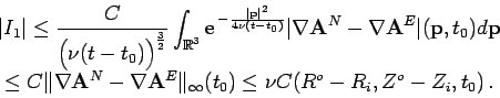
we use the Hölder inequality and end up with
,
we use the Hölder inequality and end up with
Since it is clear that ![]() is the constant function,
the proof of Lemma 2.2 will be complete when we have
shown that
is the constant function,
the proof of Lemma 2.2 will be complete when we have
shown that
![]() is homotopic to the function whose winding number is
is homotopic to the function whose winding number is ![]() ,
at least if
,
at least if ![]() ,
, ![]() , and
, and ![]() are small enough.
are small enough.
It is clear that the representation of
![]() has this property.
So let us put
has this property.
So let us put ![]() .
We need to
show that
.
We need to
show that
![]() is
small enough
to construct a linear homotopy between the representation of
is
small enough
to construct a linear homotopy between the representation of
![]() and
and
![]() that does not pass through
that does not pass through ![]() . We have already shown
this property for
. We have already shown
this property for ![]() in equation (4.3), at least when
in equation (4.3), at least when ![]() is sufficiently small. So all that remains is to show the following result.
is sufficiently small. So all that remains is to show the following result.
Proof:
We denote by ![]() the part of integral (5.1)
with
the part of integral (5.1)
with
![]() replaced by
replaced by
![]() , and by
, and by ![]() -
-![]() the parts of integral (5.1)
with
the parts of integral (5.1)
with
![]() replaced by
replaced by
![]() ;
namely by
;
namely by ![]() the integral over the inner cylinder, by
the integral over the inner cylinder, by ![]() over the cylinder
over the cylinder
![]() without the inner cylinder, by
without the inner cylinder, by ![]() the integral over the
outer cylinder
the integral over the
outer cylinder ![]() minus the cylinder
minus the cylinder ![]() and finally by
and finally by
![]() over the complement of the outer cylinder.
over the complement of the outer cylinder.
Evidently, ![]() since
since ![]() . Let us now consider
. Let us now consider ![]() .
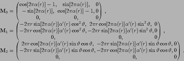
If we rewrite
.
If we rewrite
![]() (in Cartesian components)
into the cylindrical coordinates, we get that it is equal to
(in Cartesian components)
into the cylindrical coordinates, we get that it is equal to
![]() with
with
The heat kernel is independent of the angle ![]() ; after integration over
it the matrix
; after integration over
it the matrix
![]() disappears and from
disappears and from
![]() we are left with integrals of the type
we are left with integrals of the type
![\begin{displaymath}
\frac{C}{(t-t_0)^{\frac 32} \nu^{\frac 32}} \int_{\index {\b...
...2}{4\nu (t-t_0)}} r^2
\sin [2\pi \alpha (r)] \alpha '(r) dr dz
\end{displaymath}](img199.png)

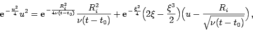
Now the application of the Taylor theorem on the function
![]() yields
yields
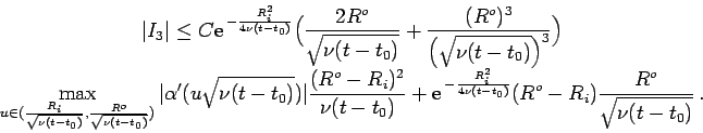
Similarly we can estimate ![]() ; here
; here
![]() are odd functions in
are odd functions in ![]() and thus we get zero after the integration of
the
and thus we get zero after the integration of
the ![]() variable.
For the components
variable.
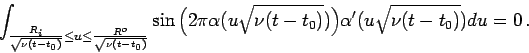
For the components ![]() ;
; ![]() proceed similarly as above and end up with
the following integral
proceed similarly as above and end up with
the following integral
![\begin{displaymath}
\int_\Omega {\rm e}\,^{-\frac{u^2+v^2}{4}}
u^2 \sin \Bigg(2...
..._0)\Big]}\Bigg) \alpha '\Big(u\sqrt {\nu(t-t_0)}
\Big) d u d v
\end{displaymath}](img218.png)
Finally,