Properties of the operator $\Gamma$

We will not prove the smoothness of solution to (1.7); it can be done in a very standard way, using the estimates to parabolic equations given for example in [5]. Let us only summarize the main result here. This will show that the function $F$ described in Lemma 2.2 is continuous on any compact subset of $[0,\infty)\times[0,2\pi]$.

Lemma 3.1   Let ${\mathbf{u}}\in C^\infty_0([0,T)\times \mbox{\Bbbb R}^3)$ for some $T>0$. Then, in the class of functions $V_k= \{{\mathbf{v}}\in L^2((0,T); L^{2}_{loc}(\mbox{\Bbbb R}^3)); {\mathbf{v}}-... ...artial {\mathbf{v}}}{\partial t} \in L^2((0,T); W^{k-2,2} (\mbox{\Bbbb R}^3))\}$, $k\geq 2$, there exists exactly one solution to (1.7). Moreover, this solution is smooth, that is, in $C^\infty((0,T]\times \mbox{\Bbbb R}^3) \cap C([0,T]\times \mbox{\Bbbb R}^3)$, and $\mathbf{A}^N-{\mathbf{x}}\in L^2((0,T); W^{k,2}(\mbox{\Bbbb R}^3))$ for any $k\geq 0$. Furthermore the solution depends smoothly upon the choice of ${\mathbf{u}}$.

Remark 3.1   Note that if ${\mathbf{u}}$ belongs to $L^\infty((0,T); L^{2}(\mbox{\Bbbb R}^3))$ $\cap L^2((0,T); W^{1,2}(\mbox{\Bbbb R}^3))$ $\cap L^1((0,T); L^{\infty}(\mbox{\Bbbb R}^3))$ (the usual information about a weak solution to the Navier-Stokes equations), then only $\mathbf{A}^N-{\mathbf{x}}\in L^\infty((0,T); W^{1,2}(\mbox{\Bbbb R}^3)) \cap L^... ...; W^{2,2}(\mbox{\Bbbb R}^3)) \cap L^\infty((0,T); L^{\infty}(\mbox{\Bbbb R}^3))$ and $\frac {\partial \mathbf{A}^N}{\partial t} \in L^2((0,T); L^{2}(\mbox{\Bbbb R}^3))$. The proof is essentially the same as the proof of Lemma 3.1 using [5] and is left as an exercise.

Lemma 3.2   There exists an interval $(0,t)$ such that for ${\mathbf{u}}$ and $\mathbf{A}^N$ smooth as in Lemma 3.1, ${\mathbf{Q}}$ is a smooth solution to (1.8).

Proof: The existence of the solution can be shown using the Galerkin method combined with standard a priori estimates. We leave the details of the proof to the reader as an exercise. width7pt height7pt depth0pt

Now, on the time interval from Lemma 3.2 we see that

$$\mathbf{Z}= (\nabla \mathbf{A}^N) {\mathbf{Q}}- {\mathbf{I}}$$

obeys the equation (see [2])

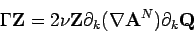$$\Gamma \mathbf{Z}= 2\nu \mathbf{Z}\partial_k(\nabla \mathbf{A}^N)\partial_k {\mathbf{Q}}$$ (3.1)

in $\mbox{\Bbbb R}^3 \times (0,T)$ with the initial condition $\mathbf{Z}({\mathbf{x}},0) = {\mathbf {0}}$. Since, for $\nabla^2 \mathbf{A}^N$ and $\nabla {\mathbf{Q}}$ bounded, there exists the unique solution to (3.1), we have $\mathbf{Z}\equiv {\mathbf {0}}$ and thus ${\mathbf{Q}}= (\nabla \mathbf{A}^N)^{-1}$ pointwise.

Also, we are now in a position to prove Lemma 2.1. Since (1.7) are uniquely solvable, it follows that the solution is axisymmetric and hence we can apply the following result.

Lemma 3.3   Let ${\mathbf{F}}: \mbox{\Bbbb R}^2 \mapsto \mbox{\Bbbb R}^2$ be a vector field which is of the class $C^1$ on some neighborhood of the origin and, written in polar coordinates, $F_r$ and $F_\vartheta$ are independent of $\vartheta$. Then

$$\frac {\partial F_x({\mathbf {0}})}{\partial x} = \frac {\pa... ...tial y} = -\frac {\partial F_y({\mathbf {0}})}{\partial x}\, .$$

Proof: Denote $F_r = f(r)$ and $F_\vartheta = g(r)$. Then we get

$$\frac {\partial F_x}{\partial x} = f' \cos^2 \vartheta + \fr... ...cos \vartheta + \frac{g}{r} \sin \vartheta \cos \vartheta \, .$$

Since $\lim_{r\to 0} \frac {\partial F_x}{\partial x}$ exists, necessarily

$$\lim_{r\to 0} \Big(f'(r) - \frac{f(r)}{r}\Big) = 0 \qquad \m... ... \qquad \lim_{r\to 0} \Big(g'(r) - \frac{g(r)}{r}\Big) = 0\, .$$

Thus $\frac {\partial F_x({\mathbf {0}})}{\partial x} = f'(0)$. Next

$$\frac {\partial F_y}{\partial y} = f' \sin^2 \vartheta + \fr... ...a \cos \vartheta - \frac{g}{r} \sin \vartheta \cos \vartheta$$

and also $\frac {\partial F_y({\mathbf {0}})}{\partial y} = f'(0)$. Analogously we get that $\frac {\partial F_x({\mathbf {0}})}{\partial y} = -g'(0)$ and $\frac {\partial F_y({\mathbf {0}})}{\partial x} = g'(0)$. The lemma is proved. width7pt height7pt depth0pt